Intro

In the world of algorithms, the first thing we would talk about is sorting. How we can sort a set of elements in a certain order? How long it takes to sort a set with a huge number of elements in it? To answer these questions we should be aware of most common sorting algorithms and its running time. There are two types of sorting algorithms, the slower one that could take Ɵ(n^2) time, and the faster one could take Ɵ(n log n) time. In this report, we shall discuss those types of algorithms and compare between them with different list sizes and the running time for each of them.

Data

1. Prepare the code to produce the following:

   • Random Array.
   • Sorted Array.
   • Reversed Sorted Array.
   • Three Semi-Sorted Arrays (20% – 50% – 80%) of the elements out of its place.
   • Bubble Sort.
   • Insertion Sort.2
   • Selection Sort.
   • Merge Sort.
   • Modified Merge Sort this modified version implement the merge sort but on the linked list.
   • Quick Sort.
   • Randomized Quick Sort.
   • Built-in Sort.

   We used C++ as our programming language to implement the functions that produced all of the above. Each of the sorting functions takes the size of the array and the array itself as an input. Then, we start with N = 10000 and increment each time 10000 up to N = 200000. Now we have 20 arrays with different sizes.

2. Calculate the running time for each sort algorithm with each of the arrays and produce six directories represents 6 different arrays that mentioned before. Each directory contains 8 files, each file contains 20 lines, and each line contains 2 space separated values. The first one the size of the array and the second value represents the running time that took from the sorting algorithm.

3. Create Python file by which we can read the data and plot the graph to show us the curve for each sorting algorithm. We used some Python libraries to load and manipulate the data. The following libraries must be installed to run Graph.py:

   • Pandas.
   • Numpy.
   • Matplotlib.

import pandas as pd
import numpy as np
import matplotlib.pyplot as plt
plt.style.use('bmh')

# Legents list required to present each line with its color in the graph.
legends = ['Merge Sort', 'Quick Sort', 'Modified Merge Sort' , 'Randomized Quick Sort', 'Build_in c++', 'Insertion Sort', 'Selection Sort', 'Bubble Sort']
col_names = ['array_size', 'time_spent']

# The following line print available plot styles; just for fun :D 
print(plt.style.available)

# Read data from the files and turn it into data frames to plot the graph.
def show_graph():
    merge_data = pd.read_csv('merge.txt', sep=' ', names=col_names)
    quick_data = pd.read_csv('quick.txt', sep=' ', names=col_names)
    inser_data = pd.read_csv('insertion.txt', sep=' ', names=col_names)
    mod_merge = pd.read_csv('modded_merge.txt', sep=' ', names=col_names)
    rand_quick = pd.read_csv('rand_quick.txt', sep=' ', names=col_names)
    selec_data = pd.read_csv('selection.txt', sep=' ', names=col_names)
    bubble_data = pd.read_csv('bubble.txt', sep=' ', names=col_names)
    build_cpp = pd.read_csv('cpp.txt', sep=' ', names=col_names)

    # Convert each dataframe into numpy array.
    merge_tm = np.array(merge_data['time_spent'])       # Merge Sort
    merge_sz = np.array(merge_data['array_size'])

    quick_tm = np.array(quick_data['time_spent'])       # Quick Sort
    quick_sz = np.array(quick_data['array_size'])

    mod_merge_tm = np.array(mod_merge['time_spent'])    # Modified Merge Sort
    mod_merge_sz = np.array(mod_merge['array_size'])

    rand_quick_tm = np.array(rand_quick['time_spent'])  # Randomized Quick Sort
    rand_quick_sz = np.array(rand_quick['array_size'])

    build_cpp_tm = np.array(build_cpp['time_spent'])    # Build in Sort in c++
    build_cpp_sz = np.array(build_cpp['array_size'])

    inser_data_tm = np.array(inser_data['time_spent'])  # Insertion Sort
    inser_data_sz = np.array(inser_data['array_size'])

    selec_data_tm = np.array(selec_data['time_spent'])  # Selection Sort
    selec_data_sz = np.array(selec_data['array_size'])

    buble_data_tm = np.array(buble_data['time_spent'])  # Bubble Sort
    buble_data_sz= np.array(buble_data['array_size'])

    # Plot the graph that containing required info.
    plt.plot(merge_sz, merge_tm)
    plt.plot(quick_sz,quick_tm)
    plt.plot(mod_merge_sz, mod_merge_tm)
    plt.plot(rand_quick_sz, rand_quick_tm)
    plt.plot(build_cpp_sz, build_cpp_tm)
    plt.plot(inser_data_sz, inser_data_tm)
    plt.plot(selec_data_sz, selec_data_tm)
    plt.plot(buble_data_sz, buble_data_tm)

    plt.grid(True)
    plt.title('Reversed sorted Array')
    plt.legend(legends, loc='upper left')
    plt.ylabel('Time (ms)')
    plt.xlabel('Array Size')
    # plt.xlim(-10, 20000) # Reduce y scale just to show more details
    plt.yscale('log')

    plt.show()

show_graph()

Outcomes

1. Random Arrays

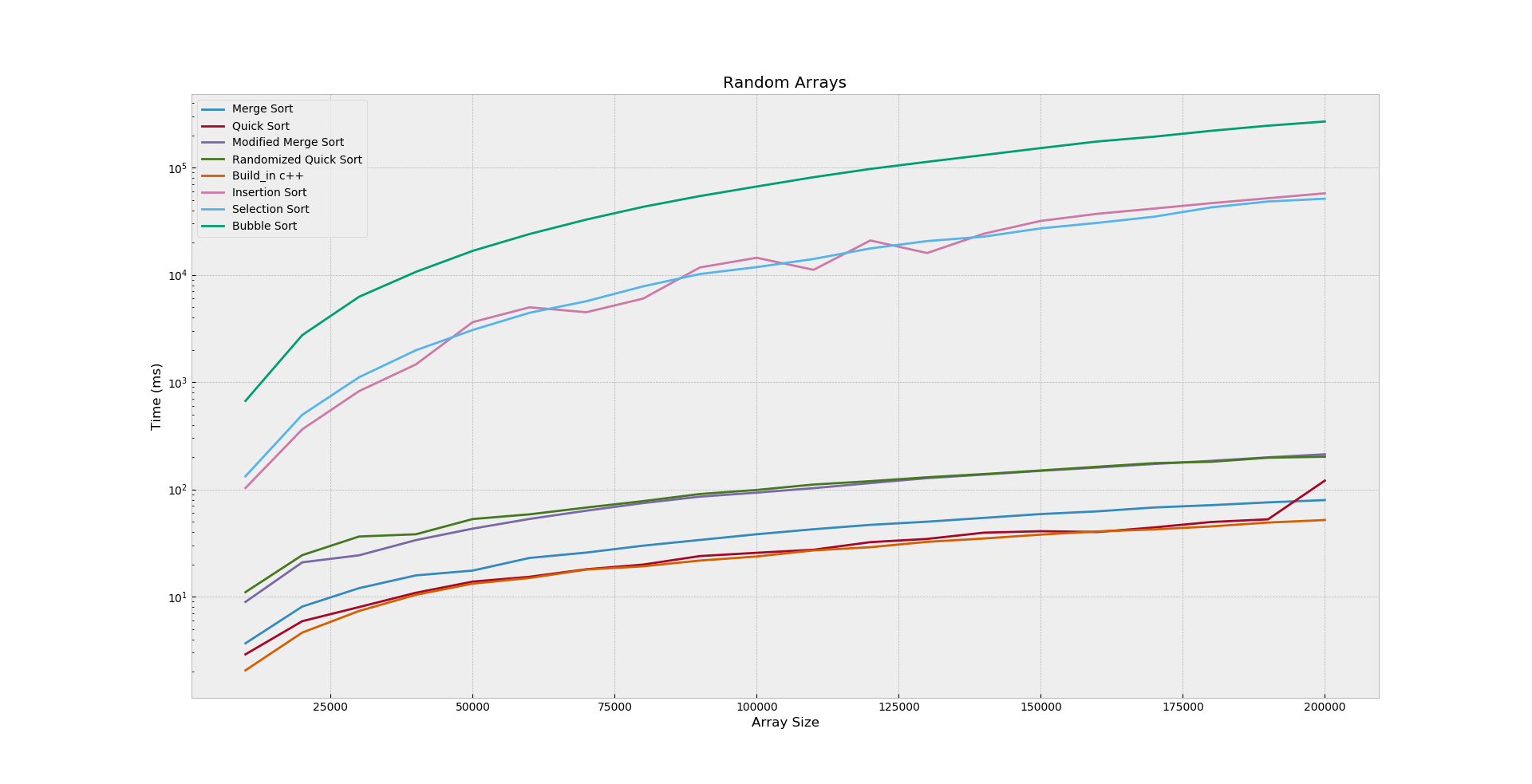
In the Figure_1, bubble sort is bad choice it takes so much time and grows quickly. Selection sort and Insertion sort almost grows together with average 29.95 (ms), the above three algorithms is almost Ɵ(n^2). The other five algorithms are less in time, the Modified Merge sort and Randomized Quick sort are larger because of randomization process and handling pointers in the linked list. It’s obvious that Merge sort, Quick sort and Built-in C++ sort is a better choice for random arrays with Ɵ(n log n) running time.

2. Semi-Sorted Arrays

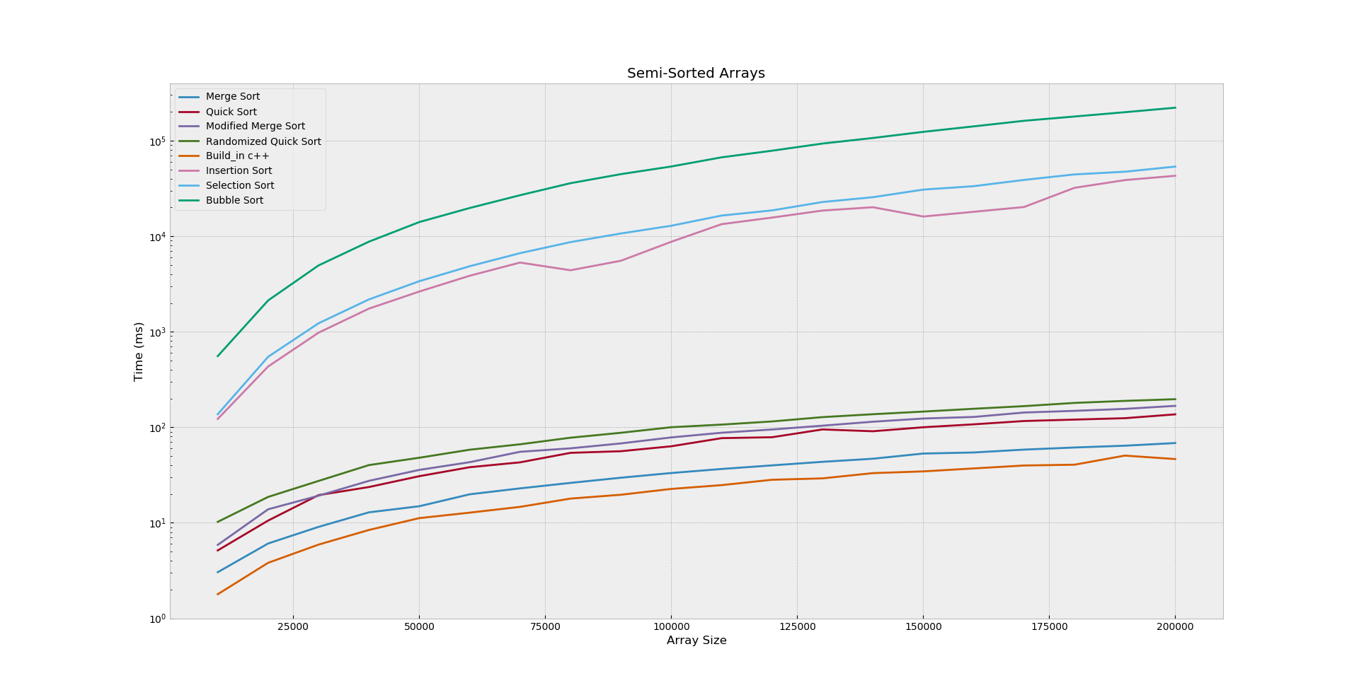
In the Figure_2, bubble sort is also a bad choice it takes so much time and grows quickly. Selection sort and Insertion sort almost grows together with average 29.95 (ms), the above three algorithms is almost Ɵ(n^2). The other five algorithms are less in time, the Modified Merge sort and Randomized Quick sort are larger because of randomization process and handling pointers in the linked list. It’s obvious that Merge sort, Quick sort and Built-in C++ sort is also a better choice for semi-sorted arrays Ɵ(n log n) running time.

3. Sorted Arrays

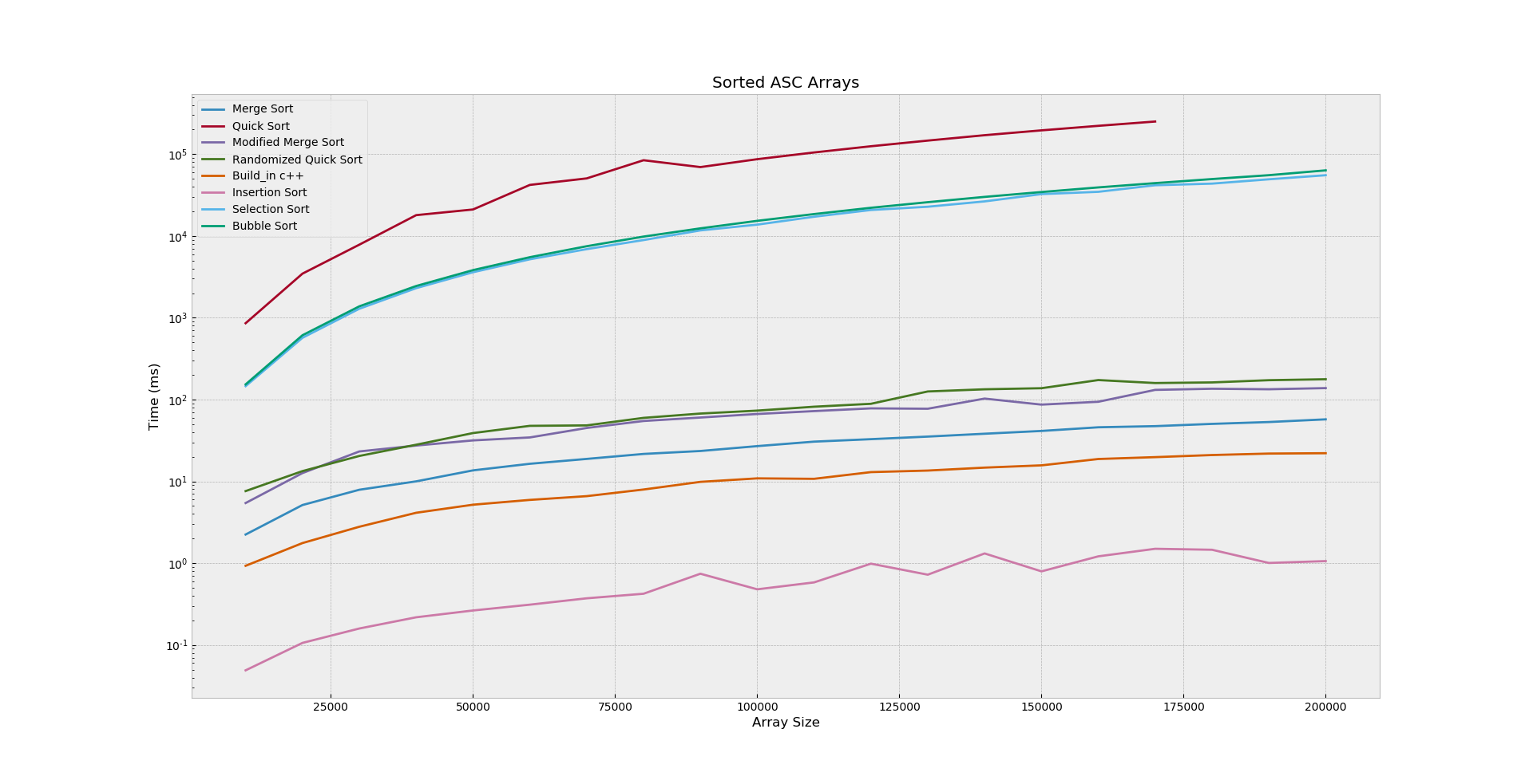
Unlike the previous figures, the Figure_3 show us the Quick sort is the worst in this case, slower than selection and bubble sort. The Modified Merge sort and Randomized sort are less in running time because of randomization process and handling pointers in linked list. Insertion sort is almost 0.99 (ms) in all sizes and it’s faster than Built-in C++. It’s obvious that Insertion sort is the best choice for sorted arrays with Ɵ(n) running time.

4. Reversed Sorted Array

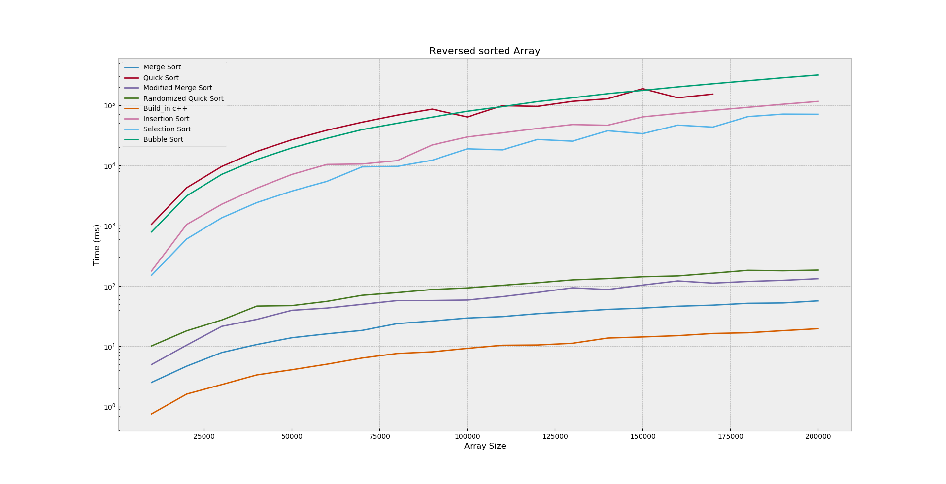
Figure_4 show us the same lines as in the sorted arrays, but the Insertion sort was unlucky it grows with Ɵ(n^2) running time.

Conclusion

As we discussed above the most common sorting algorithms used in different types of lists. If the list contains random elements we can use the Built-in or Quick sort, it’s more efficient, less in memory and less in running time from other sorting algorithms.

Insertion sort with sorted array it takes almost Ɵ(n) running time. Quick sort with sorted list or reversed sorted list it takes Ɵ(n^2) running time. Because of iterate n through (n-1) and it’s simple to calculate T(n) = T(n-1) + Ɵ(1) for both kinds.

So, it depends on what kind of lists you have, but in the real world, we insert element in place. We don’t have to sort just take an element and put it into its right place and that takes Ɵ(n) to shift other elements after inserting the picked one.

Notes:

All collected data produced by 4-core processor, so it might be slightly different if we use another higher computer to run the program. And it might be fast enough to get better results, but the running time for each algorithm will be the same.